
Bob Holt
Thursday, December 19, 2013 | 3 minutes
Generative Art - Failed Experiment 1
I’m taking Andrew Ng’s Machine Learning course on Coursera. At the same time, I’ve been thinking a lot about digital art and creative coding. I decided to try to combine the two.
This is the result.
I consider this a failure, not because it isn’t interesting, but simply because it didn’t turn out in the way I had anticipated.
The most recent assignment I completed in the machine learning course involved using Octave/MatLab to read an image, break it down to an N-Dimensional array of RGB values for each pixel, run a principal component analysis to find the important bits, and recombine them.
My idea was to take two pieces of art, break them down, and recombine them using the other work’s key, hopefully resulting in something vaguely familiar, but completely different from either work.
It didn’t turn out that way.
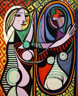
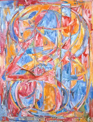
I picked two pieces somewhat off the top of my head. I was looking for pieces with a lot of color, different styles, but roughly the same aspect ratio (breaking them down into numerical matrices and swapping, requires the matrices to be of the exact same dimensions).
I ended up choosing Picasso’s Girl before a Mirror and Jasper Johns’ 0 through 9.
It turned out that there’s no discernible difference when you recombine the image using the other image’s eigenvectors. I don’t know if this is due to the limited number of dimensions in my data (3 columns in the matrix, corresponding to Red, Green, and Blue values in each pixel), a misunderstanding on my part how the eigenvectors work, or a coding error.
However, I did find that if you “normalize” the data (in the manner of
x = (x - mean(X)) / stdev(x - mean(X)) where X is the entire data set and x
is a single point in that set), you get values for each point that turns the
image into a really vivid primary-color-heavy version of itself. In this case,
the PCA step is unnecessary - it’s not doing anything for us.
This in itself wasn’t that interesting, but I was getting tired, so I wrote some code to just take the average of the two images for every pixel. This ends up creating a kind of double-exposure effect, which when combined with the vivid colors is at least a vaguely interesting result.
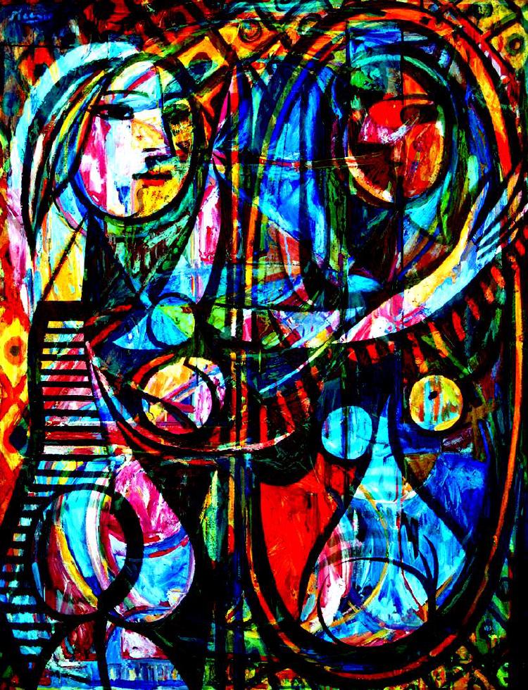
It took me about 2 hours of playing around to get an effect I could have done in 2 minutes in Photoshop. But hey, I’ve got some code I can reuse for other experiments.
Oh. here’s the code (MatLab is expensive, but Octave is free (though less friendly)):
vividmean.m
%% Initialization
clear ; close all; clc

%  Load images.
%  Images are necessarily the same pixel size.
P = double(imread('girl_before_a_mirror.jpg'));
J = double(imread('0_through_9.jpg'));

%  Normalize X by subtracting the mean value from each feature
%  and dividing by the standard deviation
P_norm = featureNormalize(P);
J_norm = featureNormalize(J);

%  Write out normalized image data
imwrite((P_norm + J_norm) ./ 2, 'vividmean.jpg');
featurenormalize.m
% Code by Andrew Ng - provided in Coursera Machine Learning Course
% https://www.coursera.org/course/ml
function [X_norm, mu, sigma] = featureNormalize(X)
%FEATURENORMALIZE Normalizes the features in X
%   FEATURENORMALIZE(X) returns a normalized version of X where
%   the mean value of each feature is 0 and the standard deviation
%   is 1. This is often a good preprocessing step to do when
%   working with learning algorithms.

mu = mean(X);
X_norm = bsxfun(@minus, X, mu);

sigma = std(X_norm);
X_norm = bsxfun(@rdivide, X_norm, sigma);


% ============================================================

end