
Bob Holt
Friday, December 20, 2013 | 4 minutes
Generative Art - The Interim Steps
Re: my previous post, there were some questions about the eigenvectors I had created, and what had happened with them when I tried to reconstruc the images.
I’ll attempt to illustrate that here.
Note that I may not show ALL of the code. Some of the functions I called are part of the assignments for the Coursera Machine Learning course (and are actually this week’s assigments), and we’ve been asked not to make those solutions public. If you really want to see the implementations, pinky-swear that you’re not taking the course, and I’ll email them to you.
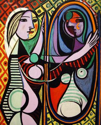
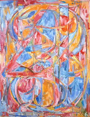
So back to the beginning. Once again, here are our original images:
So let’s look at the first part of the code. The very first part is just like in the previous post:
%% Initialization
clear ; close all; clc

%  This program Runs Principal Component Analysis on 2 images.
%  The eigenvectors of the images are swapped, and the images
%  reconstituted from the swapped eigenvectors.
%
%  Images are necessarily the same pixel size.

%  Load images
%  Values need a double datatype for matrix manipulation
P = double(imread('girl_before_a_mirror.jpg'));
J = double(imread('0_through_9.jpg'));
We clear our existing data and read in the images.
But this time, we’re going to reshape the N-dimensional vectors into 2-dimensional matrices so we can run our Principal Component Analysis:
%  Get the size of the images so we can reshape the matrix
p_img_size = size(P);
j_img_size = size(J);

%  Reshape the N-dimensional vectors representing the images' color
%  values into an Nx3 matrix where N = number of pixels.
%  Each row will contain the Red, Green and Blue pixel values
%  This gives us our dataset matrix X that we will use K-Means on.
XP = reshape(P, p_img_size(1) * p_img_size(2), 3);
XJ = reshape(J, j_img_size(1) * j_img_size(2), 3);

%  Run PCA - implementation obscured, but we run the built-in `svd`
%  function on the covariance matrix of the matrix we pass in.
%  This returns the eigenvector (U*) and eigenvalues (S*)
[UP, SP] = pca(XP);
[UJ, SJ] = pca(XJ);
All of the code up until this point will be reused in our experiments. We read in the images, translate the vectors to a 2-D matrix, and run PCA. Now comes the fun part: we need to project the images into the eigen space.
%  Project images to the eigen space using the top k eigenvectors
%  Again, the implementation is obscured, but we essentially
%  matrix-multiply our features across the first K columns of the
%  eigenvector matrix.
K = size(UP, 2); % 3
ZP = projectData(XP, UP, K);
ZJ = projectData(XJ, UJ, K);
It doesn’t make any noticeable difference which eigenvectors we use here, though they are different. They just may be so similar as to not matter:
UP =
  -0.65103   0.69800   0.29826
  -0.57221  -0.19312  -0.79704
  -0.49873  -0.68956   0.52513

UJ =
  -0.64694   0.69146   0.32149
  -0.54319  -0.12199  -0.83070
  -0.53518  -0.71204   0.45452
Finally, we recover images by reversing our projection and writing the results to disk. It’s here that I tried recovering each image using the other’s eigenvectors, to no noticeable change:
%  Recover images from the eigen space using the top K eigen vectors and
%  visualize only using those K dimensions
%  Once again, the implementation is obscured, but we reverse projectData
%  by multiplying the projected data by the same

XP_rec  = recoverData(ZP, UP, K);
XP_recovered = reshape(XP_rec, p_img_size(1), p_img_size(2), 3);

XP_swap  = recoverData(ZP, UJ, K);
XP_swapped = reshape(XP_rec, p_img_size(1), p_img_size(2), 3);

XJ_rec  = recoverData(ZJ, UJ, K);
XJ_recovered = reshape(XJ_rec, j_img_size(1), j_img_size(2), 3);

XJ_swap  = recoverData(ZJ, UP, K);
XJ_swapped = reshape(XJ_rec, j_img_size(1), j_img_size(2), 3);

imwrite(uint8(XP_recovered), 'picasso_orig.jpg');
imwrite(uint8(XP_swapped), 'picasso_swap.jpg');
imwrite(uint8(XJ_recovered), 'johns_orig.jpg');
imwrite(uint8(XJ_swapped), 'johns_swap.jpg');
But as you can see, there’s no discernable difference:


Now we can do some interesting things by reducing the number of components we use to project and rebuild the images (the K value above). There’s still no difference when we go to reconstruct, so I’ll just show each image once from now on.
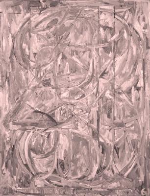
What if we reduce K from 3 (the size of the eigenvector matrix) to 2? We get
kind of a neat muted palette:


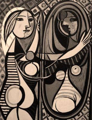
And when K = 1, we get a pretty good grayscale.
We can also do some interesting color shifting by transposing our eigenvector matrices at certain times.
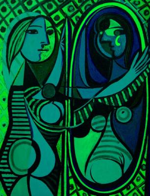
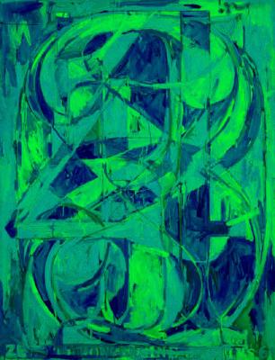
If we transpose when we project the data (when K = 3), we get a huge green shift:
ZP = projectData(XP, UP', K);
ZJ = projectData(XJ, UJ', K);
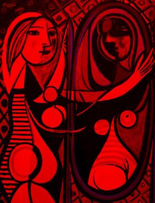
Alternately, if we transpose the matrix when we go to recover, we get a big red shift:
XP_rec  = recoverData(ZP, UP', K);
XJ_rec  = recoverData(ZJ, UJ', K);
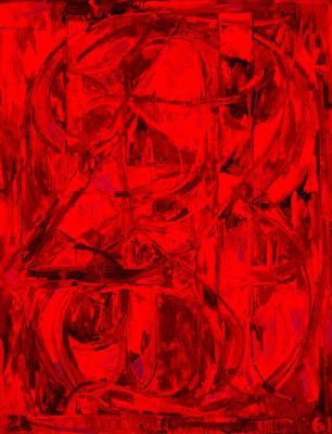
Again, nothing we couldn’t have done in a few seconds in Photoshop, but pretty fun to play with, at least.